AN ALTERNATIVE METHOD FOR FINDING KEY DRIVERS IN CUSTOMER SATISFACTION SURVEY DATA

William D. Neal

Mark E. Peterson

Presented at the Advanced Research Techniques Forum

1995

Background

In order to uncover the key drivers of customer satisfaction, many researchers regress the ratings of satisfaction with individual attributes against a rating of overall satisfaction. Typically, this procedure is fraught with challenges. The two most daunting challenges are that 1.) the dependent variable (overall satisfaction) is often heavily skewed toward the higher side of the scale and in many cases is bi-modal or even tri-modal, and 2.) there are often extreme levels of multicollinearity between the independent variables (i.e. individual attribute ratings). See Peterson et. al. (1991) for a more detailed discussion.

Interestingly, much of the current literature on customer satisfaction measurement and modeling focuses on overcoming these issues with alternative measurement scales. Although scaling is an important consideration in customer satisfaction research, we believe much of this debate is misdirected, and that in many cases a change in modeling procedures addresses the problems better.

To overcome the first challenge (skewness and multi-modality of the dependent variable), this paper advocates the use of discriminant function analysis. To overcome the second challenge (multicollinearity), this paper advocates the use of principal components analysis and a re-weighting of the principal components loading matrix. These two procedures, used in tandem, provide an alternative method for uncovering the key drivers of customer satisfaction gleaned from survey data.

This modeling approach has been used in over thirty different product and service categories since 1989 with very good results. This paper will discuss the model in detail and show the results from an actual (disguised) study.

Model Overview

The model statistically relates a single measure (rating) of overall satisfaction to a set of specific performance measures (ratings). The relationship of each performance measure to overall satisfaction is stated as an index or percentage. The index represents the relative influence of each performance measure on moving dissatisfied customers to being satisfied, or moving satisfied customers to being extremely satisfied. If a firm improves its ratings on a measure with a high index value, that will move more people from one level to the next than will an equal improvement on a lower indexed measure.

A basic assumption of the model is that the level of a customer's satisfaction falls into one of two or three possible groups:

* DISSATISFIED - meaning the customer's expectations were not met.

* SATISFIED - meaning the customer's expectations were met.

* EXTREMELY SATISFIED-meaning the customer's expectations were exceeded.

When there are only two groups (i.e., the distribution of overall satisfaction scores is bi-modal), the extremely satisfied group is usually dropped, although we have seen at least one case were there were so few dissatisfied respondents that we dropped that group.

Statistically, we are not interested in explaining (or modeling) a metric distribution of how satisfied a customer may be. Rather, we are interested in modeling the cutting planes between groups. That is, we seek to explain what performance measures differentiate either dissatisfied from satisfied, or satisfied from extremely satisfied. We name these two models as follows.

The ZERO DEFECTS MODEL addresses the performance measures that differentiate dissatisfied customers from satisfied customers, ignoring those who are extremely satisfied. If a firm concentrates its resources on eliminating defects that differentiate dissatisfied customers from satisfied ones, then they will drive the number of customers that are dissatisfied toward zero. Alternatively, some of our clients have chosen to name this model the BARRIERS TO SATISFACTION MODEL.

The EXCELLENCE MODEL addresses the performance measures that differentiate satisfied customers from extremely satisfied customers, ignoring those that are dissatisfied. If a firm concentrates its resources on eliminating defects that differentiate satisfied customers from extremely satisfied ones, then it will maximize the number of customers that are extremely satisfied. Alternatively, some of our clients have chosen to name this model the BARRIERS TO LOYALTY MODEL - assuming extremely satisfied customers are also loyal customers. Recognizing that that assumption is being challenged in some quarters, we will continue to refer to this model as the Excellence Model.

There is also a very valid managerial rationale for addressing two models in customer satisfaction. We have observed many times that those performance measures that highly differentiate dissatisfied customers from satisfied ones are often quite different, or at least have very different importances (weights), than those that differentiate satisfied customers from extremely satisfied customers - in fact, that is one reason why regression across the entire distribution can be most misleading. For example, if a hotel customer experiences a reasonably efficient check-in, a clean, neat, safe room where everything works properly, and a reasonably efficient checkout, they are usually satisfied. Therefore, these performance measures are the key ones that differentiate a satisfied customer from a dissatisfied one. On the other hand, what differentiates a satisfied customer from an extremely satisfied one may include such things as speed of room service, friendliness of the staff, availability of business service facilities, and so forth. These latter items would show very little differentiation (or importance) in the ZERO DEFECTS model, but would typically show much more differentiation (importance) in the EXCELLENCE model.

A basic tool of our analysis is, therefore, discriminant function analysis (DFA) - a multivariate statistical technique for finding an optimal cutting plane between two distributions. DFA assumes that each group category (e.g. dissatisfied and satisfied) is really a measure of a central tendency of a normal distribution of the degree of dissatisfaction or satisfaction. DFA then finds the least squares plane that optimally separates those two distributions. The cutting plane is expressed as a multivariate linear model. The DFA weights from the model, one for each performance factor, indicate the degree to which that factor separates the two groups. In the ZERO DEFECTS model, the DFA weights can be interpreted as measures of what the firm is doing to keep dissatisfied customers from being satisfied. In the EXCELLENCE model, the weights can be interpreted as measures of what the firm is doing to keep satisfied customers from being extremely satisfied.

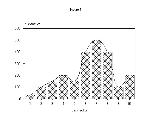
Graphically, an illustrative distribution of overall satisfaction of customers, measured on a 10-point scale, may look like Figure 1 below.

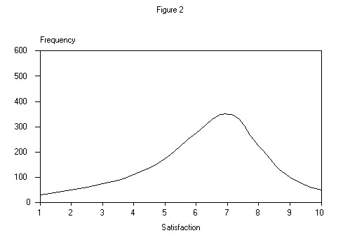
The majority of the literature on customer satisfaction measurement (see Peterson et al.) assumes this distribution is a theoretically continuous one that is typically skewed to the left as shown in Figure 2 below.

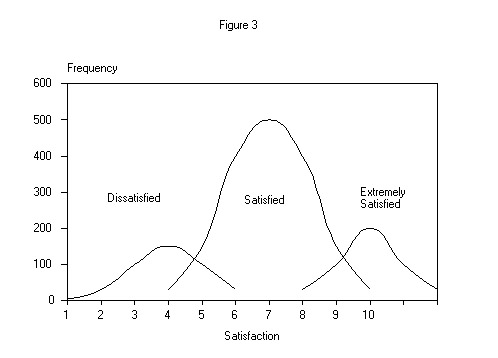
On the other hand, we believe a frequency distribution of this type is more often the convergence of (two or) three nearly normal distributions of (two or) three populations - dissatisfied, satisfied, and extremely satisfied customers - as shown in Figure 3 below.

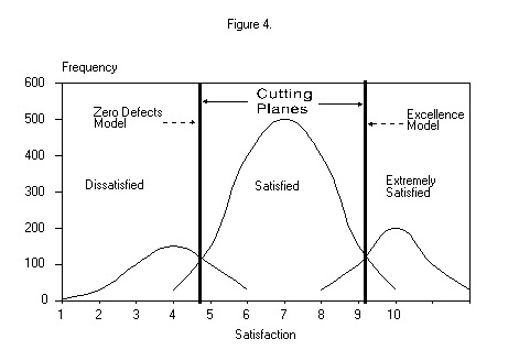
Thus, we assume that there are (one or) two optimal cutting planes that will discriminate between the (two or) three populations and reveal those performance measures that differentiate the populations as shown in Figure 4 below.

Although a particular firm's distribution of customer satisfaction may not match the one shown in Figure 1, typically at least one optimal cutting plane can be found in the distribution. DFA allows us to test the degree of separation between the distributions, test the predictive reliability using a holdout sample, and then determine to what degree each performance measure contributes to this separation or differentiation, although not directly, as will be seen shortly. It is not unusual for the model to attain an 80% or better correct classification of a holdout sample.

The model requires that overall customer satisfaction be measured either one of two ways. One way is to use a direct 3-point scale - dissatisfied (did not meet expectations), satisfied (just met expectations), extremely satisfied (exceeded expectations.) Alternatively, you may use a 9-point or greater scale, explicitly show the distribution (as in Figure 1), and use DFA to find the optimal cutting plane(s).

Performance Measures and Multicollinearity

Turning to the individual performance measures, we assume that all of them, in combination, represent an exhaustive set of those aspects of the firm's performance which would have a significant influence on a customer's level of overall satisfaction. The appropriate set of performance measures is usually unique to each product/service category. The identification of the appropriate set of performance measures requires front-end research with current and previous customers. Often, focus groups, customer interviews, and "closed account" surveys are used to develop the exhaustive set of performance measures.

The performance measures should be made using metric (equal - interval) scales. We prefer eleven-point or similar scales in order to optimize measures of variance.

Ideally the set of independent variables in CSM surveys should be just that - independent. It is rare that they are. Principal components analysis (PCA) with a VARIMAX rotation is often used to assess the level of multicollinearity among the set of independent performance measures. Using each principal component as a "scale", it is rather simple to conduct a reliability analysis and eliminate redundant and non-contributing performance measures. However, this process often eliminates some of the more action-oriented performance measures and makes any subsequent reporting of the influence of all performance measures difficult.

Our strategy for dealing with multicollinearity is to aggregate the performance measures into a smaller set of uncorrelated substitute measures which we call PERFORMANCE FACTORS using standard Principal Components Analysis (PCA) with a VARIMAX rotation.

Once we have defined the performance factors from the PCA, we calculate the raw loading (correlation) of each performance measure on each performance factor (principal component) for each respondent. Thus, we may start with, say, 50 performance measures. Then we may define, say, 10 performance factors with PCA which explain 70% or more of the variance in the original set of performance measures. We then calculate each respondent's score on each of the 10 performance factors. These 10 scores become the independent predictor variables in the DFA discussed previously.

The resulting correlations of performance factors to the discriminant function (W_k) are used to weight the "loadings" (i.e. squared correlations - r²_jk) of individual performance measures to the performance factors. The weighted squared correlations are then summed across rows to give an overall "importance" for the performance measure, I_j. This is graphically shown in Figure 5.

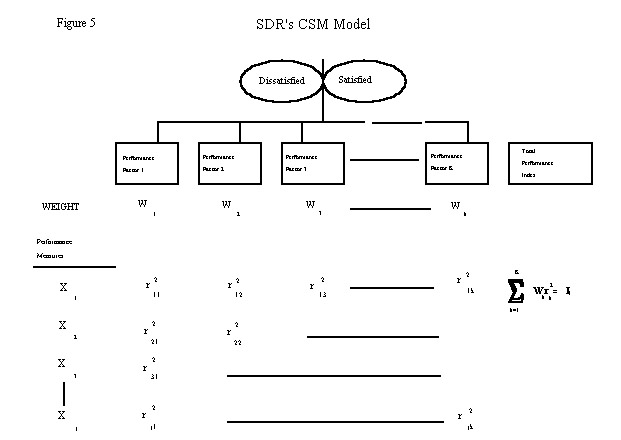
where:

Xj  = Performance Measure j.

Wk  = Correlation of performance factor k on the discriminant function

The Total Importance Index, which is expressed as a percentage for each importance measure, provides a relative value of the importance of that measure in differentiating two satisfaction groups, say, dissatisfied customers from satisfied customers.

An improvement in the firm's performance on a high indexed performance measure will have a greater impact on moving customers from being dissatisfied to being satisfied then will an equal improvement on a performance measure that has a lower index.

Table 1. shows a disguised (and incomplete) example from a Cable Television study - ACE Cable Company's market segment D.

Table 1.

ACE CABLE COMPANY

MARKET SEGMENT D

Realistically, the performance measures tend to clump together as they typically do in the real environment. That is, one would expect "Quality Programs" and "Picture Reception" to load heavily on the "Value for the Money" performance factor, and management may typically address these two measures in concert.  This effect can be easily seen by inspecting the loadings of those two performance measures on the performance factor "Value for the Money."

However, some performance measures may load significantly on more than one performance factor. And, because they do so, they may accumulate a higher importance index. In this example the performance measure "Timely Response" loads heavily on all five performance factors, giving it an overwhelming overall importance. In this study, open-ended questions verified that the cable company's customers were extremely frustrated by the inability of the company to schedule a particular time for an installation or repair, and also that when appointments were made, they were not always kept.

Given the above, it is important to consider (1) each performance factor, as an underlying construct of service and performance, 2) the weight the performance factor has on the level of satisfaction, (3) the performance measures that load heavily on each performance factor, noting especially those that load significantly on more than one performance factor, and (4) the overall order of the indices, before taking definitive action to improve customer satisfaction.

Caveats and Considerations

Data Considerations and Requirements